Background Estimation using Simple Moving Average in Python
To perform quantitative calculations from data such as spectra, it is effective to remove the background in advance. While simple methods like linear approximation can sometimes be used to estimate the background, in cases of complex background shapes, it can be challenging.
In such cases, a useful method is to repeatedly apply a simple moving average to process the data such as spectra and estimate the background. This entry explains this method.
This method is also implemented in sablib, a C++ library for smoothing and baseline estimation. Please feel free to check it out if you are interested.
Properties of the simple moving average
The simple moving average is a method in which, for any arbitrary point $(x_{i}, y_{i})$ and its neighboring $N$ points $(x_{i-N}, y_{i-N}), \dots, (x_{i}, y_{i}), \dots, (x_{i+N}, y_{i+N})$, the average value is calculated,
$$
\displaystyle
\bar{y}_{i} = \frac{1}{2N+1}\sum^{N}_{j=-N}y_{i+j}
$$
and $y_{i}$ is replaced with $\bar{y}_{i}$, and this process is repeated. It is sometimes used to smooth data containing noise. In this case, increasing $N$ suppresses noise more strongly, but at the same time, side effects become stronger.
Here is an example of applying a simple moving average to data containing peaks.
(blue line: original data; orange line: simple moving average with small $N$; gray line: simple moving average with large $N$)
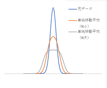
Since each point taking the average has an equal weight, points near the peak are strongly influenced by the peak area, while the peak area is strongly influenced by the background. As a result, the peak becomes smaller and transforms into a shape with a broader base.
Estimation of Background
In utilizing a simple moving average for estimating the background, this property is exploited. By purposely taking a large $N$ for the simple moving average, the peaks are smoothed out. Then, by comparing the smoothed data with the original data and selecting the smaller value, it is defined as the new data (1). (blue line: original data; gray line: simple moving average; red line: new data)
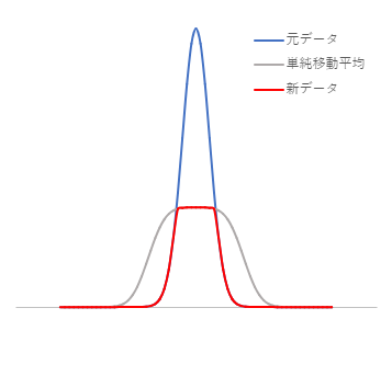
Take a simple moving average again on the new data (1), compare it with the new data (1), select the smaller value, and define it as the new data (2). By repeating this process, the peaks will eventually be smoothed out to a level similar to that of the background.
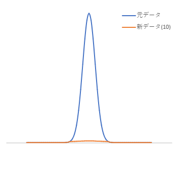
Here is an example of repeating this process 10 times. It can be seen that the peaks have been smoothed out near the background. If repeated a few more times, it seems reasonable to consider it as part of the background. (blue line: original data; orange line: new data after 10 times repeated)
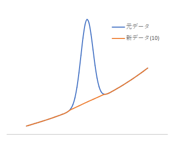
This method can be effectively used in relatively flat regions, even if the background is not perfectly flat. Below is an example of applying this method to peaks with a gentle curve background. The process has been repeated 10 times here as well. (blue line: original data; orange line: new data after 10 times repeated)
This method is convenient because it can be processed relatively quickly. However, users are left to decide how many times to repeat the operation and what value to set for $N$. Since it depends on the data, making a decision can be challenging. For example, in the reference document [1], it is mentioned that setting $N$ to 2-4 times the FWHM of the peak is typical.
Application to Data Containing Noise
In the above explanation, we used smooth data, but in real-world data, it often contains noise components. When applying the above method to original data containing noise, I conducted an experiment to see how it would turn out.
The original data is a pseudo-spectrum with added white noise to smooth data containing multiple synthesized peaks from an arbitrary function, with 1000 data points. For this data, the operation of taking a simple moving average with $N=20$ was repeated 20 to 100 times. The data points at both ends within $N$ were left unprocessed, preserving the original data.
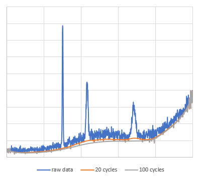
From the results, it seems that repeating the operation 20 times is sufficient for estimating the background well. Additionally, it was observed that overly smoothing the peak-shaped background by repeating the process too many times could lead to underestimating the background. It appears that more repetitions do not necessarily result in a better outcome.
Furthermore, since the method involves taking the lower value between the moving average and the original data, in the case of data containing noise, the background is adjusted to the lower level of the noise. Therefore, preprocessing the spectrum with methods such as the Savitzky-Golay filter or Whittaker Smoother beforehand may lead to better estimation of the background.
Reference
Implementation in Python
I implemented the above operations in Python. You can write the code very concisely as shown below.
Simple moving average can be easily implemented using convolve() from Numpy. Additionally, element-wise comparisons can be done in one line using Numpy.
import numpy as np

def estimate_background_with_moving_average(y, points, cycles):
    n = 2 * points + 1
    y_tmp = y.copy()

    for i in range(cycles):
        y_old = y_tmp.copy()
        y_tmp[points:-points] = np.convolve(y_old, np.ones(n) / n, mode='valid')
        y_tmp = np.where(y_tmp > y_old, y_old, y_tmp)

    return y_tmp
Conclusion
I introduced a method for estimating the background using a simple moving average. To summarize the process:
- Take a simple moving average with an arbitrary number of points $N$ and compare it with the original data.
- Select the smaller value and define it as the new data.
- Apply step 1 to the new data again.
- Repeat this process a suitable number of times.
As shown above, you can achieve this relatively easily in Python. It may not be too complex in other languages without powerful libraries like Numpy.