Improvement of AsLS method – implementation of airPLS and arPLS methods in C++
In a previous article, I introduced a background estimation method using Asymmetric Least Squares Smoothing (AsLS), which utilizes the Whittaker Smoother. In this article, I would like to introduce improved versions of the AsLS method: adaptive iteratively reweighted Penalized Least Squares (airPLS) and asymmetrically reweighted Penalized Least Squares (arPLS).
The airPLS method and arPLS method are also implemented in sablib, a C++ library for smoothing and baseline estimation. Please feel free to check it out if you are interested.
Review of the AsLS Method
For details on the AsLS method, please see the following article:
Background Estimation by Asymmetric Least Squares Smoothing (AsLS) in C++
The AsLS method is a technique that smooths out peaks by repeatedly applying the Whittaker Smoother:
$$
\displaystyle
Q = \sum_{i}w_{i}(y_{i} – z_{i})^{2} + \lambda\sum_{i}(\Delta^{s}z_{i})^{2}
\tag{1}
$$
Here, $w_{i}$ is the weight, $\lambda$ is the penalty coefficient, and $s$ is the number of differences. To make the second term, which represents roughness, dominant, a deliberately large value is given to the penalty coefficient $\lambda$ to crush the peaks.
The Whittaker Smoother is applied again after comparing with the original data. At this time, the weight $w_{i}$ is changed according to the result of the comparison with the original data. Using a weight parameter $p$, a weight of $w_{i} = p$ is given to points where $y_{i} > z_{i}$, and conversely, a weight of $w_{i} = 1 – p$ is given to points where $y_{i} <= z_{i}$. This means that the importance of points where the original data is larger than the smoothed data is reduced. By doing this, only the data near the baseline gradually remains. The iterative calculation is terminated when the weight $w_{i}$ no longer changes.
The AsLS method is a relatively simple and powerful technique, but it also has its challenges. One is how to set the parameter $p$. Also, since a uniform weight of $w_{i} = p$ is given to points where $y_{i} > z_{i}$, the importance of points where $y_{i} > z_{i}$ is significantly reduced, even if they are actually part of the background. As a result, the background is fitted to the low level of the noise.
The airPLS and arPLS methods introduced in this article are techniques that address these issues.
airPLS and arPLS methods
airPLS method
The airPLS method is an improved version of the AsLS method published by Zhang et al. in 2010 [1]. The author’s manuscript and implementations in MATLAB, R, and Python are available on GitHub.
In the airPLS method, the weight $w_{i}$ is determined as follows:
$$
w_{i} =
\begin{cases}
0 & y_{i} \geqq z_{i} \\
e^{\frac{t|y_{i} – z_{i}|}{|\mathbf{d}|}} & y_{i} < z_{i}
\end{cases}
$$
Here, $t$ is the number of iterations, and $\mathbf{d}$ is a vector containing only the points where $y_{i} < z_{i}$. When $y_{i} \geqq z_{i}$, the weight is set to 0, so these points are excluded from the next calculation. On the other hand, when $y_{i} < z_{i}$, the weight $w_{i}$ is calculated by an exponential function. Since the value of the exponent is 0 or greater, the weight $w_{i}$ is expected to be 1 or greater. From this, in the airPLS method, the importance of points where $y_{i} \geqq z_{i}$ becomes zero, and the importance of points where $y_{i} < z_{i}$ becomes higher than in the AsLS method.
Incidentally, the absolute value symbol is confusing, but looking at the author’s Python implementation, $|\mathbf{d}|$ is:
dssn = np.abs(d[d < 0].sum())It is calculated as the absolute value of the sum of the points where $y_{i} < z_{i}$. It should be noted that this is not the magnitude of the vector.
Also, in the paper, the numerator of the exponent of the exponential function is $t(y_{i} – z_{i})$. However, looking at the author’s Python implementation:
w[d < 0] = np.exp(i * np.abs(d[d < 0]) / dssn)
w[0] = np.exp(i*(d[d < 0]).max() / dssn)
w[-1] = w[0]
It actually takes the absolute value (I have corrected it to the absolute value in this article). Furthermore, the weights at both ends are calculated differently. This is not apparent without looking at the implementation.
The convergence is determined by the following formula:
$$
|\mathbf{d}| < 0.001 \times |\mathbf{y}|
$$
This convergence criterion formula is very confusing. Looking at the author’s Python implementation, the convergence criterion part is:
dssn < 0.001 * (abs(y)).sum()While $|\mathbf{d}|$ was the "absolute value of the sum", $|\mathbf{y}|$ is the "sum of the absolute values". This would also be impossible to know without the author’s implementation.
The airPLS method is often used as a benchmark in papers on baseline estimation methods. While the importance of points where $y_{i} \geqq z_{i}$ is eliminated, the importance of points where $y_{i} < z_{i}$ becomes even higher than in the AsLS method, so the problem of the background being fitted to the low level of the noise remains.
arPLS method
The arPLS method is an improved version of the AsLS method published by Baek et al. in 2015 [2]. The author’s manuscript is available.
In the arPLS method, the weight $w_{i}$ is determined as follows:
$$
w_{i} =
\begin{cases}
\frac{1}{1 +\exp\left({\frac{2(d_{i} – (-m_{\mathbf{d}^{-}}+2\sigma_{\mathbf{d}^{-}}))}{\sigma_{\mathbf{d}^{-}}}}\right)} & y_{i} \geqq z_{i}\\
1 & y_{i} < z_{i}
\end{cases}
$$
Here, $d_{i} = y_{i} – z_{i}$. When $\mathbf{d} = \mathbf{y} – \mathbf{z}$, a vector consisting only of the parts where $y_{i} < z_{i}$ is defined as $\mathbf{d}^{-}$. $m_{\mathbf{d}^{-}}$ and $\sigma_{\mathbf{d}^{-}}$ are the mean and standard deviation of $\mathbf{d}^{-}$, respectively.
The exponential function part is complex, but this function is a logistic function. The logistic function is a function with an S-shaped curve and is widely used in statistics. It has the characteristic of taking values between 0 and 1. arPLS uses this characteristic for weighting.
Even in the region where $y_{i} \geqq z_{i}$, a relatively large weight is given where the difference between $y_{i}$ and $z_{i}$ is small, such as noise on the baseline, and a value close to 0 is given where the difference is large, such as at a peak. This addresses the problem of the background being fitted to the low level of the noise.
The convergence is determined by the following formula:
$$
\frac{|\mathbf{w}^{t} – \mathbf{w}^{t + 1}|}{|\mathbf{w}^{t}|} < ratio
$$
The weights are updated, and the difference with the previous weights is calculated. The calculation terminates when the ratio of the magnitude of this difference to the magnitude of the previous weights becomes smaller than a certain value.
References
Implementation example with Eigen
The airPLS method has implementations in MATLAB and Python on the author’s GitHub, and the arPLS method also has MATLAB code in reference [2], so it is relatively easy to implement it yourself. Based on these, I implemented it in C++ and Eigen.
I have also published the code on GitHub, so please take a look if you are interested. Note that whittaker.h, whittaker.cpp, and diff.h are required for building. These codes are also available on GitHub. Please download them together.
airPLS method
- airpls.h
#ifndef __IZADORI_EIGEN_AIRPLS_H__
#define __IZADORI_EIGEN_AIRPLS_H__

#include "whittaker.h"

// Background estimation by airPLS method
//
// y       : Actual observation data
// lambda  : Penalty coefficient for smoothing
// diff    : Order of difference (1-3)
// maxloop : Maximum number of iterations
// loop    : Actual number of iterations (return value)
const Eigen::VectorXd BackgroundEstimation_airPLS(
    const Eigen::VectorXd & y, const double lambda, const unsigned int diff,
    const unsigned int maxloop, unsigned int & loop
);

#endif // __IZADORI_EIGEN_AIRPLS_H__- airpls.cpp
#include "airpls.h"

const Eigen::VectorXd BackgroundEstimation_airPLS(
    const Eigen::VectorXd & y, const double lambda, const unsigned int diff,
    const unsigned int maxloop, unsigned int & loop
)
{
    size_t m = y.size();

    loop = 0;
    Eigen::VectorXd w(m), z, d;
    double y_abs_sum, d_sum_abs;

    w.setOnes(m);
    y_abs_sum = y.array().abs().matrix().sum();

    while (loop < maxloop)
    {
        z = WhittakerSmoother(y, w, lambda, diff);

        d = (y.array() >= z.array()).select(0, y - z);
        d_sum_abs = std::fabs(d.sum());

        // Convergence check
        if (d_sum_abs < 0.001 * y_abs_sum)
        {
            break;
        }

        // Update weight w
        loop++;
        w = (y.array() >= z.array()).select(0, ((loop * d.array().abs()) / d_sum_abs).exp());
        w(0) = w(w.size() - 1) = std::exp((loop * d.maxCoeff() / d_sum_abs));
    }

    return z;
}
arPLS method
- arpls.h
#ifndef __IZADORI_EIGEN_ARPLS_H__
#define __IZADORI_EIGEN_ARPLS_H__

#include "whittaker.h"

// Background estimation by arPLS method
//
// y       : Actual observation data
// lambda  : Penalty coefficient for smoothing
// ratio   : Threshold for convergence check
// maxloop : Maximum number of iterations
// loop    : Actual number of iterations (return value)
const Eigen::VectorXd BackgroundEstimation_arPLS(
    const Eigen::VectorXd & y, const double lambda, const double ratio,
    const unsigned int maxloop, unsigned int & loop
);

#endif // __IZADORI_EIGEN_ARPLS_H__- arpls.cpp
#include <limits>
#include "arpls.h"

const Eigen::VectorXd BackgroundEstimation_arPLS(
    const Eigen::VectorXd & y, const double lambda, const double ratio,
    const unsigned int maxloop, unsigned int & loop
)
{
    size_t m = y.size();

    loop = 0;
    Eigen::VectorXd w(m), wt, z, d, tmp;
    double mean, sd;
    Eigen::Index ct;

    // Overflow prevention
    const double overflow = std::log(std::numeric_limits<double>::max()) / 2;

    w.setOnes(m);

    while (loop < maxloop) {
        z = WhittakerSmoother(y, w, lambda, 2);

        d = y - z;

        ct = (d.array() < 0).count();
        mean = (d.array() < 0).select(d, 0).sum() / ct;
        sd = std::sqrt((d.array() < 0).select((d.array() - mean).matrix(), 0).squaredNorm() / (ct - 1));

        tmp = ((d.array() + mean - 2 * sd) / sd).matrix();
        tmp = (tmp.array() >= overflow).select(0, (1.0 / (1 + (2 * tmp).array().exp())).matrix());

        // Update weight w
        wt = (d.array() >= 0).select(tmp, 1);

        // Convergence check
        if ((w - wt).norm() / w.norm() < ratio) {
            break;
        }

        w = wt;
        loop++;
    }

    return z;
}
In the arPLS method, the content of the exponential function tends to become a large value, which can easily cause an overflow. Therefore, a countermeasure has been implemented. The maximum value for which the exponential function does not overflow is determined by taking the logarithm of the maximum value of double, and if the content of the exponential function exceeds this value, the result of the logistic function is set to 0.
Environment confirmed to work
- OS
- Windows 10
- Microsoft C/C++ Optimizing Compiler 19.44.35207.1 for x64
- MinGW-W64 GCC version 13.2.0
- Clang version 20.1.0
- Linux
- GCC version 12.2.0
- Windows 10
- Eigen version 3.4.0
Application to data containing noise
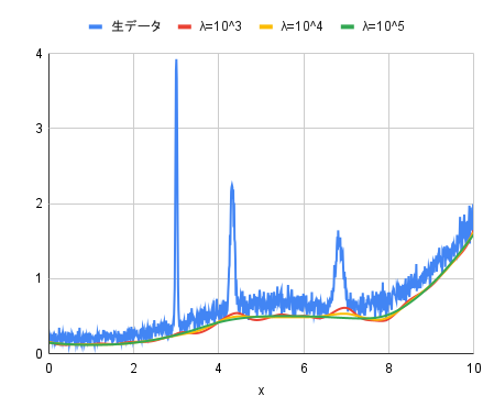
Using the code above, I experimented by applying it to data containing noise to see what kind of background would be generated.
The original data is a pseudo-spectrum with 1000 data points, created by adding white noise to smooth data containing multiple peaks synthesized from appropriate functions.
For this data, I evaluated the cases where $\lambda$ was set to $10^{3}, 10^{4}, 10^{5}$ for both the airPLS and arPLS methods. The other parameters were set to a difference order diff of 2 for the airPLS method, and a convergence criterion ratio of 0.001 for the arPLS method.
- airPLS method
- arPLS method
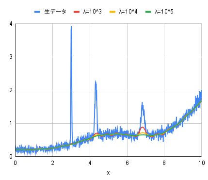
For both the airPLS and arPLS methods, the cleanest background seems to be drawn when $\lambda$ is $10^{5}$.
The difference between the two is the height of the background. While the airPLS method fits the background to the low level of the noise, the arPLS method fits the background to the center level of the noise. The arPLS method seems to provide a more natural baseline.
Summary
I have introduced background estimation using the airPLS and arPLS methods. The summary of their operation is as follows.
- airPLS method
- Apply the Whittaker Smoother with a large $\lambda$. All weights are set to 1.
- Compare with the original data, set the weight of points where $y_{i} \geqq z_{i}$ to 0, and for other points, set it to $e^{\frac{t|y_{i} – z_{i}|}{|\mathbf{d}|}}$.
- Apply the Whittaker Smoother again.
- Repeat step 2 until $|\mathbf{d}| < 0.001 \times |\mathbf{y}|$ is satisfied.
- arPLS method
- Apply the Whittaker Smoother with a large $\lambda$. All weights are set to 1.
- Compare with the original data, set the weight of points where $y_{i} \geqq z_{i}$ to $\frac{1}{1 +\exp\left({\frac{2(d_{i} – (-m_{\mathbf{d}^{-}}+2\sigma_{\mathbf{d}^{-}}))}{2\sigma_{\mathbf{d}^{-}}}}\right)}$, and for other points, set it to 1.
- Apply the Whittaker Smoother again.
- Repeat step 2 until $\frac{|\mathbf{w}^{t} – \mathbf{w}^{t + 1}|}{|\mathbf{w}^{t}|} < ratio$ is satisfied.