Background Estimation by Asymmetric Least Squares Smoothing (AsLS) in C++

2024-01-232024-07-16Background,Baseline,C++,Eigen,Signal Processing,Spectrum

In the previous article, I introduced a method for estimating the background using a simple moving average. In this article, I would like to introduce Asymmetric Least Squares Smoothing (referred to as AsLS or ALS), a background estimation method using Whittaker Smoother, which is explained in Whittaker Smoother.

1. Propaties of Whittaker Smoother
2. Principle of AsLS Method
- 2.1. Reference
3. Implementation using C++ and Eigen
- 3.1. Operating Environment
- 3.2. Application to Data Containing Noise
4. Conclusion

Propaties of Whittaker Smoother

Please refer to the following article for information on Whittaker Smoother:

Implementation of Whittaker Smoother in C++ with Eigen

One widely used method for smoothing data containing noise such as spectra is the Savitzky-Golay ...

https://izadori.net/en/math-whittaker-en/

In summary, when considering fitting a smooth data sequence $\boldsymbol{z}$ to an observed measurement data sequence $\boldsymbol{y}$, it leads to a penalized least squares problem with two elements: the goodness of fit of $\boldsymbol{z}$ to $\boldsymbol{y}$, and the roughness of $\boldsymbol{z}$.

$$
\displaystyle
Q = \sum_{i}w_{i}(y_{i} – z_{i})^{2} + \lambda\sum_{i}(\Delta^{s}z_{i})^{2}
\tag{1}
$$

Here, $w_{i}$ represents weights, $\lambda$ is the penalty coefficient, and $s$ is the number of differences. While we will consider the weights $w_{i}$ later, let’s focus on the penalty coefficient $\lambda$ for now. For the purpose of smoothing, $\lambda$ is usually set to a relatively small value, such as 1. However, let’s examine the behavior when an extremely large value is deliberately set for $\lambda$.

The second term in equation (1) relates to roughness. Increasing $\lambda$ makes the roughness term dominant, leading to an even smoother line. Below are the results of applying a Whittaker Smoother with a large $\lambda$ to a simple Gaussian peak ($s = 2$). (blue line: original data)

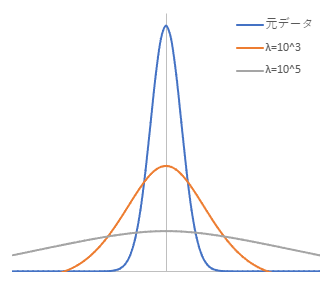
As can be seen from the figure, increasing $\lambda$ causes the peak to decrease and the shape to transform into a broader base, deviating from the original curve. This behavior is similar to the characteristics of a simple moving average. The AsLS method also utilizes this property.

Principle of AsLS Method

In the method that utilizes the AsLS algorithm, unlike the approach in estimating background using a simple moving average, weights $w_{i}$ are utilized. Specifically, a weight parameter $p$ is introduced, where for points where $y_{i} > z_{i}$, the weight $w_{i} = p$ is assigned, and for points where $y_{i} <= z_{i}$, the weight $w_{i} = 1 - p$ is assigned. The Whittaker Smoother is then applied again. This process is repeated until the weights $w_{i}$ no longer change.

The idea behind this is to assign a smaller weight $p$ to points where $y_{i} > z_{i}$, which are considered to be areas where the peaks have been smoothed out, thereby reducing the importance of smoothing and giving higher importance to points closer to the baseline where $y_{i} <= z_{i}$. This leads to the generation of a smooth curve that fits points closer to the baseline.

$p$ should be a small value, hence it is set to less than 0.5. According to Eilers, a good choice for $p$ is $0.001 \leqq p \leqq 0.1$. Additionally, regarding $\lambda$, it is mentioned that $10^{2} \leqq \lambda \leqq 10^{9}$ is a good range (although there are exceptions), as stated in a paper by Eilers[1].

Reference

Eilers, P. H. C.; Boelens, H. F. M. Baseline Correction with Asymmetric Least Squares Smoothing Leiden University Medical Centre Report2005, 1(1), 1-5.

Implementation using C++ and Eigen

In reference [1], there is MATLAB code provided, making it relatively easy to implement the algorithm on your own. Based on this, I implemented the algorithm in C++ using Eigen. However, the code is fixed with 10 iterations, so some modifications are necessary to make it more general (Eilers mentions that 5-10 iterations are sufficient). For added flexibility, I made it possible to set the number of iterations.

I have also published the code on GitHub, so feel free to check it out if you are interested. Additionally, you will need to include whittaker.h, whittaker.cpp, and diff.h for building the code. These files are also available on GitHub for download.

asls.h

#ifndef __IZADORI_EIGEN_ASLS_H__
#define __IZADORI_EIGEN_ASLS_H__

#include "whittaker.h"

// Background estimation by AsLS method 
//
// y       : observed data
// lambda  : penalty coefficient
// p       : weights
// maxloop : maximum iteration number
// loop    : actual iteration number(return value)
const Eigen::VectorXd BackgroundEstimation_AsLS(
  const Eigen::VectorXd & y, const double lambda, const double p,
  const unsigned int maxloop, unsigned int & loop
);

#endif // __IZADORI_EIGEN_ASLS_H__

asls.cpp

#include "asls.h"

const Eigen::VectorXd BackgroundEstimation_AsLS(
  const Eigen::VectorXd & y, const double lambda, const double p,
  const unsigned int maxloop, unsigned int & loop
)
{
  size_t m = y.size();

  loop = 0;
  Eigen::VectorXd w, w0, z, pv(m), npv;

  w.setOnes(m);
  w0.setZero(m);
  pv.fill(p); npv = (1 - pv.array()).matrix();

  while(loop < maxloop)
  {
      z = WhittakerSmoother(y, w, lambda, 2);

      // update weights vector w
      w = (y.array() > z.array()).select(pv, npv);

      // Check the end of iteration
      if(((w.array() - w0.array()).abs() < 1e-6).all())
      {
          break;
      }

      w0 = w;
      loop++;
  }

  return z;
}

Operating Environment

OS
1. Windows 10
  1. Microsoft C/C++ Optimizing Compiler 19.28.29913 for x64
  2. MinGW-W64 GCC version 8.1.0
  3. Clang version 11.0.1
2. Linux
  1. GCC version 9.3.0
Eigen version 3.3.9

Application to Data Containing Noise

I conducted an experiment using the code mentioned above to apply it to data containing noise and observe the type of background generated.

The original data consists of a pseudo-spectrum created by synthesizing multiple peaks within a smooth data, with white noise added, and has 1000 data points. I evaluated this data with $\lambda$ set to $10^{3}, 10^{6}, 10^{9}$. $p$ was set to 0.01, and the maximum number of iterations was set to 100.

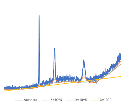
From the results, it can be seen that with $\lambda = 10^{3}$, the background estimation for the peak areas is significantly overestimated, while with $\lambda = 10^{9}$, the background deviates greatly. It seems that setting $\lambda$ too high is not ideal. In this case, $\lambda = 10^{6}$ provided a good estimation for the background.

The convergence for each case was 5 iterations, 6 iterations, and 6 iterations, respectively.

Conclusion

I have introduced the background estimation using the Asymmetric Least Squares (AsLS) method. A summary of the process is as follows:

Apply Whittaker Smoother with a large $\lambda$, giving a weight of 1 to all points.
Compare with the original data, assign a weight parameter $p$ for points where $y_{i} > z_{i}$ and $1 – p$ for other points.
Apply Whittaker Smoother again.
Repeat step 2 until all weights $w_{i}$ stop changing.

As shown in the implementation example, using Eigen in C++, including the Whittaker Smoother part, can be implemented with relatively short code. However, determining the optimal values for parameters such as $\lambda$ and $p$ poses a challenge, requiring trial and error to find the best values.

There have been many improved methods based on the AsLS method, and I hope to introduce some of these methods in the future.

Background,Baseline,C++,Eigen,Signal Processing,Spectrum

Posted by izadori